1. Information About the Muller Method:

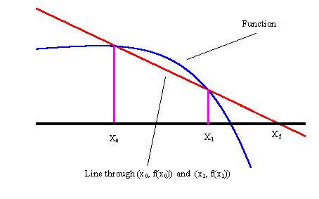
This method was first presented by D.E. Muller in 1956. This technique can be used for any root finding program but it is particularly useful for approximating the roots of polynomials. Muller method’s is an extension of the Secant Method. The secant method begins with the two initial approximations x₀ and x₁ and determines the next approximation x₂ as the intersection of the x-axis with the line through (x₀, f(x₀)) and (x₁, f(x₁)).

Figure.1: The Secant Method.

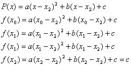
But the Muller Method uses the three initial approximations x₀, x₁, x₂ and determines the next approximation X₃ by considering the intersection of x-axis with the parabola through (x₀, f(x₀)), (x₁, f(x₁)) and (x₂, f(x₂)). This can be seen in the following figure. Then the following can be written:

Figure.2: f(x) and the Interpolating Polynomial for Muller’s Method.

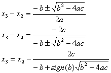
After arranging the above equations we get the following :

Then X₃ can be found easily by using the formulas that are used for calculating the roots of parabolas. The following lines explain this:

The power of Muller Method comes from the fact that it finds the complex roots of the functions. This property makes it more useful when compared with the other methods. (like Bisection, Newton, Regula-Falsi …)

2. The General Pseudo Code for the above Mathematical Formulas :

INPUT x₀ , x₁, x₂ ; tolerance TOL ;

Maximum number of iterations N₀

OUTPUT approximate solution p or message of failure

Step 1 Set h₁= x₁ - x₀

h₂= x₂ – x₁

Step 2 While do steps 3-7

Step 3

( Note : Maybe Complex Arithmetic)

Step 4

If < then set E= b+D

Else set E= b-D

Step 5

Step

Step 6 If < TOL then

OUTPUT( p ) (Procedure Completed Successfully)

STOP

Step 7 Set x₀=x₁ (Prepare for next iteration)

x₁=x₂

x₂=p

h₁= x₁ - x₀

h₂= x₂ – x₁

Step 8

OUTPUT (‘Method Failed After N₀ iterations, N₀= ‘,N₀)

(Procedure Completed unsuccessfully)

STOP

3. The Algorithm for Multiple Root Finding:

The main point of the of the Multiple Root Finding is deflation. In deflation you obtain some other functions by dividing the initial one with (x-x₀) where x₀ is the found root. This can be done in a loop so that you can find many roots of a function.

But you should determine the point where the loop will be terminated. This can be done when the function becomes constant. When a function is divided with all (x-x_N) where x_N ‘s are roots of the function, the left term must be a constant. So in the loop checking whether the function becomes constant or not is enough to determine when the loop will be terminated. This can be done by calculating value of function at three points and determining if they are equal or not. If all the three values are equal it can be said that the function becomes constant. Then the loop should be terminated. But there is problem here, in computer two double numbers can very rarely be exactly equal. Then a threshold should be determined and the difference between the two values of the function should be compared with this threshold. The comparison may be relative or absolute.

4. Error and Stopping Criteria:

While implementing the algorithm two errors criteria should be considered. First of them is e where it satisfies the following :

The other one is “tol” that is given in the pseudo code provided in the part 2. Our algorithm checks both of them according to the desire of the user. In the applet if the check box is not clicked value of that error critter is set to zero. This means that the stopping critter is determined with the other checked one. The typical values for these errors are 1e-8. This value provides the user with enough accuracy in found roots.

Another stopping criteria is the maximum number of iterations provided by the user. When the number of iterations gets over this number the program terminates.

5. Problems with the Muller Method:

Two main problems may arise while implementing the Muller Method.

First problem is the fact that the three points used for interpolating the function may have the same function values. (that is f(x₀) = f(x₁) = f(x₂)). When this condition is applied to the code given in part 2, it can easily be seen that the Muller Algorithm fails. To avoid this failure in each step the values of f(x₀),f(x₁) and f(x₂) are checked if they are equal the points are perturbed.

The second problem arises when the points (x₀ ,f(x₀)) (x_{1 ,}f(x₁)) and (x₂ ,f(x₂)) are on the same line. When this happens the algorithm jumps to Secant method begins by finding real root.

6. General View of the Algorithm Used:

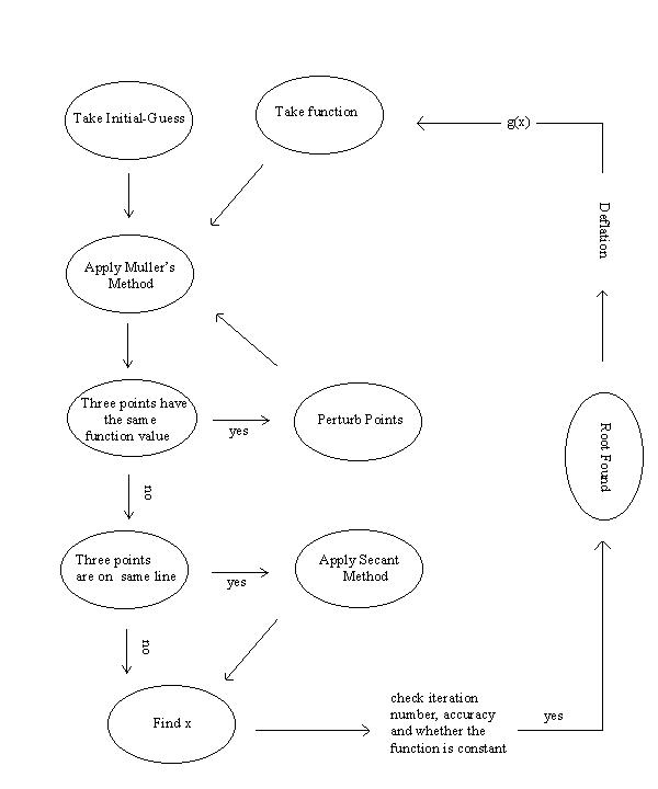
The following figure shows the general overview of the algorithm used.

Figure.3: General Overview of the Algorithm

7. Conclusions and Results:

In this section some results of the program that is the implementation of the Muller’s Algorithm will be presented. While obtaining these results the initial guess was kept as ‘0’. Both error criteria were checked in the applet. Their values were set to 1e-10. The following lines give the function and the found roots. Also the values of the function and the number of iterations at these roots are provided. Normally the results given in the applet are rounded but here to show how accurate the program is I provide them with more than required digits.

7.1 f(x) = sin(x)/x

The results are as follows:

Root#	Root(Real)	Iter. #	Real Part of f(x)	Imaginary Part of f(x)
1	3.141592653589793	7	3.898043091051478E-17	0
2	-3.141592653589793	8	-6.203928263260538E-18	0
3	-6.283185307179586	8	-1.3165144662472426E-18	0
4	9.42477796076938	13	3.142946774328553E-20	0
5	6.283185307179586	7	3.33477010006078E-20	0
6	-9.42477796076938	13	-5.307451454997275E-22	-9.394837143527715E-39
7	-12.566370614359172	16	-3.2179319401260514E-23	-4.35260386726895E-40
8	-21.991148575128552	21	-4.9792339217089986E-26	9.1281756754985E-43

Table.1: The results of sin(x)/x = 0

It can be seen that for the last three roots the imaginary part of the function is not exactly zero but very close to it. So, These are reliable results.

7.2 f(x) = (x-1)⁵⁰

The results are as follows:

Root #	Root(Real)	Iter. #	Real Part of f(x)	Imaginary Part of f(x)
1	0.9999987722510164	886	7.443409049471834E-179	-9.078588778242684E-178
2	0.9999992564343607	897	-2.1445363950872054E-179	2.9494186898034E-178
3	0.999999971973291	909	3.424893412021876E-188	-4.826112656706602E-189
4	0.9999998296846422	884	-1.5747466298356112E-183	-2.12226912708916E-184
5	0.9999999404983325	885	-9.818989340219747E-183	-4.710913124116839E-183
6	1.0000000192416685	874	-6.712055423408525E-189	1.7643543309812252E-187
7	0.9999999903652947	894	1.143990477293188E-184	4.922566557251823E-184
8	0.9999999884374289	873	-2.6014310896141423E-182	1.0332640725690462E-182
9	0.9999999897460768	883	4.898268636515677E-182	1.7916933138721888E-181
10	0.9999999961264135	873	4.8656823582055196E-178	2.720927745792945E-178
11	0.9999999963763585	865	-1.1382613422515526E-173	-6.043182115919059E-174
12	0.9999999984298037	866	1.8585453280760798E-173	-5.895104615804684E-174
13	0.999999998056031	786	-1.3875354521154783E-161	-4.074410264982218E-163
14	0.9999999979971642	757	-1.1139622202075888E-153	9.856725903636141E-155
15	0.999999998963756	704	4.808788402814985E-146	6.318573778928948E-146

Table.2: The results of (x-1)⁵⁰ = 0

7.3 f(x) = (x-1)¹⁰(x-2)¹⁰(x-10)¹⁰/(x-10)⁸

The results are as follows:

Root #	Root(Real)	Iter. #	Real Part of f(x)	Imaginary Part of f(x)
1	0.9999999995328123	458	-4.29607995651174E-92	-3.3815105697148335E-92
2	0.9999999989608178	385	-1.3700780482455824E-79	-1.6740245937034516E-79
3	0.9999999996770118	360	-9.969223618998642E-74	-1.851539196287381E-74
4	0.9999999992611898	292	-9.125409378738328E-62	2.9481866963976814E-62
5	0.9999999995157624	245	-4.567308235264821E-53	-2.2406707710538733E-53
6	0.999999999452553	197	-7.200524776703963E-44	3.668625681591965E-44
7	1.00000000018902	157	-8.131962904879378E-37	8.631038587232952E-37
8	0.9999999999892526	108	-1.0975534876595566E-27	1.0290918880740657E-28
9	1.0000000004384533	48	6.476547418865541E-20	-1.9828083340721684E-19
10	1.0000000002200646	31	4.431629895849358E-1	1.1322427272400067E-11
11	1.9999999986904577	425	-1.025968635081423E-87	-7.925283989936569E-88
12	1.999999998734595	377	-1.3023721007766524E-78	-2.4128339185309364E-78
13	1.9999999990636739	329	-4.6514196771147585E-70	-2.83349886728813E-70
14	1.999999999068222	281	-4.887011356138486E-61	-3.392922525942465E-61
15	1.9999999996489075	237	-3.158306715906007E-53	-1.731829449302457E-54
16	1.9999999999017246	203	-1.7666042152919476E-47	-4.9822577870168084E-48
17	2.0000000002435616	145	-4.538675900505214E-37	-6.787507937808772E-37
18	1.999999999943159	90	-2.3914831569182227E-27	-1.7446099206942172E-28
19	2.000000000441148	26	2.5702551449636412E-20	8.279996045034185E-20
20	2.000000000305346	9	-1.2511770848034138E-10	1.958907143872885E-10
21	10	5	-6.924504390102018E-34	-8.479792073015E-50
22	10	3	0	0

Table.3: The results of (x-1)¹⁰(x-2)¹⁰(x-10)¹⁰/(x-10)⁸ = 0

7.4 f(x) = (x³+1)¹⁵

The results are as follows:

Root#	Real Part of Root	Imag. Part of Root	Iter.#	Real Part of f(x)	Imag. Part of f(x)
1	0.49999994807196324	-0.866025346798947	515	-2.88801936E-100	-2.587779859E-101
2	0.49999994807196324	0.866025346798947	0	-2.88801936E-100	-2.587779859E-101
3	0.499999868559941	0.8660252769952951	441	-6.426191977E-88	1.33750958191E-88
4	0.499999868559941	-0.866025276995295	0	-6.426191977E-88	1.33750958191E-88
5	0.5000001868366238	0.8660253812708647	389	4.9426427570E-82	6.01304833271E-82
6	0.5000001868366238	-0.866025381270864	0	4.9426427570E-82	6.01304833271E-82
7	-0.9999997897403975	0	478	2.1472458455E-95	-3.1423537812E-95
8	0.49999989737874684	-0.86602526757991	382	-1.457346391E-75	5.19517459784E-75
9	0.49999989737874684	0.86602526757991	0	-1.457346391E-75	5.19517459784E-75
10	-0.9999997921957868	0	450	1.9558131773E-88	-2.9374676196E-88
11	0.49999985294586513	-0.866025311746580	342	1.8931793529E-68	1.63037360220E-68
12	0.49999985294586513	0.8660253117465809	0	1.8931793529E-68	1.63037360220E-68
13	-0.9999998102164986	0	405	5.0286263787E-82	-2.1984954331E-82
14	-0.9999998063035457	0	380	8.6072800865E-75	4.90736470996E-75
15	0.4999998363455767	-0.866025349786988	300	-1.086663620E-62	2.47114072117E-62
16	0.4999998363455767	0.866025349786988	0	-1.086663620E-62	2.47114072117E-62
17	0.4999998318098343	-0.866025391665197	276	-1.196309137E-56	5.61967583730E-56
18	0.4999998318098343	0.8660253916651979	0	-1.196309137E-56	5.61967583730E-56
19	-0.9999999370718109	0	375	8.2296542272E-76	-3.0337815504E-76
20	0.4999998309287459	0.866025431435627	238	-4.916225099E-50	-9.7704300129E-50
21	0.4999998309287459	-0.866025431435627	0	-4.916225099E-50	-9.7704300129E-50
22	-0.9999999506084445	0	335	7.2131105342E-70	-1.3532519110E-70
23	0.4999999690782306	0.8660252495383586	201	-2.858357234E-44	1.03901481170E-44
24	0.4999999690782306	-0.866025249538358	0	-2.858357234E-44	1.03901481170E-44
25	-0.9999998550290774	0	270	5.0211987082E-58	1.01906052688E-57
26	-0.9999999743733012	0	269	3.2721685468E-57	1.33401348222E-59
27	0.5000000614954219	0.8660253710285922	196	2.0993429140E-44	7.74313832181E-45
28	0.5000000614954219	-0.866025371028592	0	2.0993429140E-44	7.74313832181E-45
29	0.4999999876562415	0.8660254664161138	168	1.5362762370E-38	1.68537492932E-38
30	0.4999999876562415	-0.866025466416113	0	1.5362762370E-38	1.68537492932E-38

Table.4: The results of (x³+1)¹⁵ = 0

By examining the above results it can be said that the program can successfully find the roots of very high ordered functions. Also it is again successful in finding the roots of sinusoidal and oscillating functions. Further developments may be necessary for some other types of functions.

8. References

[1] Numerical Analysis, R.L. Burden, J.D. Faires, PWS Publishing Company, Boston 1993.