Wireless Propagation Simulation

Wireless Propagation Applet*

Notes: You should have Java Runtime Environment (JRE) installed in order to run this applet. (see http://java.sun.com)

Different browser types handle applets differently, so try one of the following alternative pages if you are experiencing problems.

Main Page , Alternative 1 , Alternative 2

*: Formerly known as 2-D Electromagnetic Field Analyzer (EFA)

This is a voluntary project constructed by Guray Gurel, A. Cafer Gurbuz and A. Serdar Kilinc for educational and research purposes under the supervision of Dr. Ayhan Altintas to demonstrate propagation of waves originating from wireless base stations.

This project received "The Best Educational Program Award" in Software Quest 2002.

This page and the applet code is last revised by Guray Gurel on March 4, 2004.

1. Introduction and Motivation

With the increasing use of wireless base stations in urban areas, electromagnetic power distribution and its effect on human health became an important subject. This applet demonstrates two-dimensional power analysis of electromagnetic waves radiating from these base stations with a bird's eye view of the map. The area of interest is determined by a map code whose characteristics are defined below. This map can also be generated automatically using the visual interface tools provided within the applet. Having determined the map, the code is compiled and the output is presented in a window where the magnitude of the power matrix is drawn in grayscale. The points to compute the power is determined via the usage of a sampling distance. The exact value of the power at a point (magnitude) is indicated as the mouse is moved over the map.

2. Getting to know the applet.

When the applet starts, a window opens which shows the preview of the map described by the code in the editor (fig.1). Since there is no code, the preview window is initially empty. Unless indicated otherwise, the applet assumes that the map is 20 meters to 20 meters with a sampling distance of 0.1 meters. As the user draws the map by using the three methods described below, the code in the editor and the preview changes simultaneously (see 'using the mouse to draw a map').

There is a wizard and settings panel within the applet. Using this panel, you can add sources or draw buildings just by indicating their coordinates without any need to know how to write map code. When the applet is opened "Add a Source" panel is opened by default (Fig 2). You can add or remove sources from this panel easily.

By selecting "Add a Building" part you can draw a wall or a building by giving the coordinates of the corners (Fig. 3). You can add bunch of buildings one by one from this panel. This method ensures that closed polygons are formed with the given parameters. This is important when considering the wedge angles during computing the contribution of diffraction.

The "General Settings" part allows user to change the default values of some parameters (Fig. 4). By this way one can see the effects of any parameter and maybe set the values for a special case.

3. Components of the Map

There are two different components of the map. These are sources and the walls/ buildings. These components are added to the map using one of the three methods. The parameters of these components like maximum power of a source or reflections constant of the walls can be changed from the "General Settings".

3.a) Using the Wizard to draw a map

Wizard is integrated into the applet and by default "Add a Source" is opened (Fig. 2). To add sources you just give the coordinates of the sources and add them by clicking "Add Source" button. You will see the added sources in the "Added Sources" field. From this field you can select and remove sources by "Clear Selected Source" button. After adding all the sources it is required to click the "OK" button at the bottom of the panel. Otherwise sources will not be entered to the map. After this you can see the sources in the "Map Code Area".

To add a wall/building* to the map, you have to give the coordinates of the corners and add them by clicking "Add Point" button. After adding all the corners of the building you have to press the "OK" button to finish that building. By this way you can add lots of buildings**.

See 'Changing the Wizard Settings' to see how the wizard can change the sampling distance and the size of the map.

* In this simulation, only one side of a wall is considered to be reflective in order to reduce the amount of calculation in simulations of closed polygons. Therefore, other than the coordinates of the two ends of a wall, the coordinates of a reference point, which is any arbitrary point on the non-reflecting side of the wall should be provided. The wizard calculates the reference point as the mid-point of a convex polygon. Therefore, the reference points of the walls should be modified to satisfy the original needs if an open or concave polygon is drawn.

** You should press OK button after adding all walls of the polygon into the wizard.

3.b) Using the mouse to draw a map

You can put sources and walls into the map using the mouse on the preview pane. When the applet is first started, it is in draw mode by default. In this mode, you can put sources at the points you desire by a single click. The sources you indicated will be previewed as yellow dots and corresponding codes will be automatically added to code area. You can draw walls by dragging the mouse cursor from one end to the other and of the wall. When you start dragging, you will realize a blue line indicating where the wall is going to lie. When you stop dragging by releasing the mouse button, you will realize another blue line that originates from the middle of the wall and ends at the cursor of the mouse. This latter line is a guide indicating the non-reflecting side of the wall (Only one side of a wall is intended to be reflective since our computations will involve buildings of closed polygons). Move the mouse the the non-reflecting side of the wall and click anywhere to finish the wall. The code will be added to the code area.

It is not recommended to try to draw closed polygons using mouse. Single walls have a wedge angle of 360 degrees. If the end points of single walls do not coincide, they do not form a closed polygon and hence the resulting diffraction contribution will be different than the expected one as a consequence of the unintended difference in wedge angles.

In order to change the sampling distance or the size of the map, right click the preview pane. The following menu will appear.

3.c) Writing your own code and the commands.

You can write the map code yourself by using the "Map Code" field in the applet. All the map coordinates are in meters. Anything other than a proper command will be interpreted as a comment and will not be taken into account.

Adding a Source: To add a source you only need to start with "s" and then write the X and Y coordinates respectively. For example "s 3 12" means a source which has a X coordinate of 3 and a Y coordinate of 12.

Adding a Wall: To draw a wall, you use

w X1 Y1 X2 Y2 R1 R2

where X1, Y1, X2, Y2, R1, R2 are the x coordinate of the first end, y coordinate of the first end, x coordinate of the second end, y coordinate of the second end, x coordinate of the reference point, y coordinate of the reference point, respectively. You should recall that (R1,R2) denotes the reference point which is any arbitrary point on the non-reflecting side (e.g. on the inside of a closed building). As an example:

The code of this map is:

s 5 5

w 7 8 10 8 15 15

w 11 6 16 6 10 1

Here the first 4 numbers are the corner coordinates. As we see the bottom mirrors reflecting side is the upper side. Because its reference point is "15 15", which sees the bottom side of the mirror, so the reflecting side is the other side. On the other hand the upper mirrors reflecting side is the bottom side since its reference point is "10 1". By this way you can add lots of walls. This example and the examples below do not employ diffraction.

Adding a Building: To add a polygon you have to give the required information mentioned above for every wall of the building. But you have to be careful to match the end points to close up the polygon. If you don't EFA will still work, but you may see power inside the buildings. Actually the easiest way to form a building is to give the corner coordinates by using the wizard. An example code and the map of a building is below:

s 4 11

w 4 1 7 2 5 3 As you see all the reference points are same for the walls. Because when you draw a building

w 7 2 8 5 5 3 by using the wizard, it automatically gives the same reference point for all the walls.

w 8 5 5 7 5 3

w 5 7 2 3 5 3

w 2 3 4 1 5 3

Changing the Sampling distance: To change the sampling distance, we use the command

r New_Value

where New_Value indicates the new sampling distance in meters. When there are more than one r commands in a code, the last one is effective.

Changing the Size of the Map: To change the size of the map, we use the command

z New_Width New_Height

where New_Width and New_Height are the width and the height of the map in meters respectively. When there are more than one z commands in a code, the last one is effective.

4. Changing the Wizard Settings

You can change some settings from the "General Settings". There are some different parameters that affect the power of the receiver points in this settings panel. By changing the parameters one can analyze and observe the effects of these parameters. Here we have:

Wavelength: This parameter changes the wavelength of the radiated wave which affects the phase of the power.

# of Reflections: This declares the number of the reflections before the the power of the wave dies down.

# of Diffractions: Indicates how many times a diffracted wave can be diffracted again, e.g. setting this to 1 will ensure that a diffracted ray will not experience diffraction again. It will just die if it hits another corner.

Max-Min Power: In illustrating the power distribution on the map, the power levels are colored according to these values. Power values greater than or equal to Max Power is shown in white, power levels lower than Min Power is shown in black and what remains in between is mapped linearly to the 256 shades of gray.

Reflection Constant: The reflection constant to be used in electromagnetic reflection formula. It defines the attenuation caused by a reflection on a wall.

5. Running the Code

After finishing the map by any method you want, you may press the "Compile/Run" button in the applet and wait for the calculations. The time required depends on the number of buildings and sources. The percentage of the progress will be shown. At the end the power map will appear in a grayscale form.

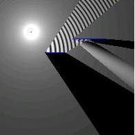
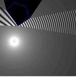
6. Analyzing the Power Map

In the map, power values larger than Max Power is indicated by white, the power values lower than Min Power is indicated as black and all what remains in between is indicated with a linear mapping from the Min-Max Power interval to the 256 shades of gray. In other words, brighter regions indicate higher power magnitudes. When you move the mouse over the power map, a window showing up at the top left of the screen will tell the magnitude of the power at the pointed location. You can change the Min-Max Power levels by right clicking the Power Map. In this case, the power map will be redrawn according to the new values you provided.